VanderPolDemo.m
Contents
Overview
This script illustrates the stiffness of the Van der Pol equation


Beginning of code
Initialize
clear all
close all
f = @(t,y,mu) [y(2); mu*(1 - y(1)^2)*y(2) - y(1)];
t0 = 0;
y0 = [2 0];    % initial condition
tol = 1e-4;
Example 1
We use  , which results in a non-stiff problem which ode23 can easily handle
tmax = 20;
mu = 0;
opts = odeset('RelTol',tol);
ode23(f,[t0 tmax],y0,opts,mu);
title(strcat('ode23 solution of van der Pol equation, \mu = ',int2str(mu)));
xlabel('time t');
ylabel('solution y');
legend('y_1','y_2')

Plot of first component (position) vs. time
pause
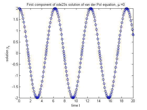
[t,y] = ode23(f,[t0 tmax],y0,opts,mu);
plot(t,y(:,1),'-o');
title(strcat('First component of ode23s solution of van der Pol equation, \mu = ',int2str(mu)));
xlabel('time t');
ylabel('solution y_1');
Solving the same problem with ode23s
pause
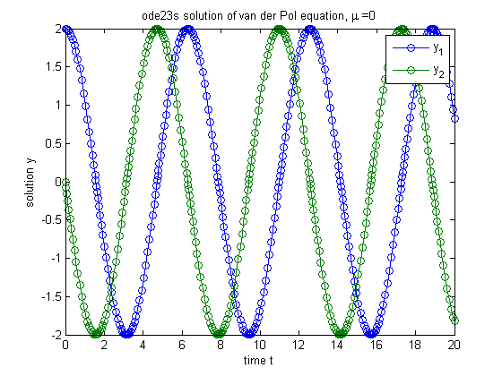
ode23s(f,[t0 tmax],y0,opts,mu);
title(strcat('ode23s solution of van der Pol equation, \mu = ',int2str(mu)));
xlabel('time t');
ylabel('solution y');
legend('y_1','y_2')
pause
Example 2
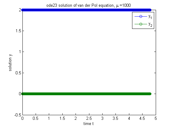
If we change  , then the problem becomes stiff, and we need see that ode23 is very slow. Note the short
  -range in the plot. The stiff solver ode23s does a much better job below.
tmax = 1000;
mu = 1000;
opts = odeset('RelTol',tol);
ode23(f,[t0 tmax],y0,opts,mu);
title(strcat('ode23 solution of van der Pol equation, \mu = ',int2str(mu)));
xlabel('time t');
ylabel('solution y');
legend('y_1','y_2')
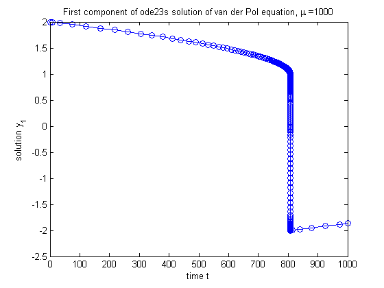
Plot of first component (position) vs. time (using ode23s)
pause
[t,y] = ode23s(f,[t0 tmax],y0,opts,mu);
plot(t,y(:,1),'-o');
title(strcat('First component of ode23s solution of van der Pol equation, \mu = ',int2str(mu)));
xlabel('time t');
ylabel('solution y_1');
Solving the same problem with ode23s
pause
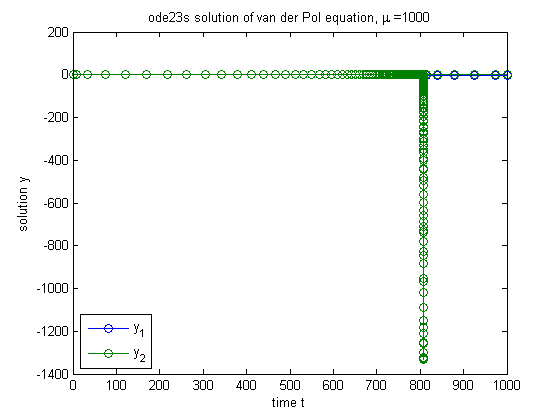
ode23s(f,[t0 tmax],y0,opts,mu);
title(strcat('ode23s solution of van der Pol equation, \mu = ',int2str(mu)));
xlabel('time t');
ylabel('solution y');
legend('y_1','y_2','Location','SouthWest')
pause
